背景 短文本question-answer匹配度识别问题,论文(Learning to Rank Short Text Pairs with Convolutional Deep Neural Networks.pdf), github实现 。github的作者基本上实现了文章里的算法,计算的精度也差不多,不过使用theano实现的,我准备使用tensorflow实现,并解决大规模预料训练太慢的问题。当然本文要开始从分析git的实现开始讲起,会穿插theano的一些语法,实现等,我自己也是从零学起的,且当给自己留个笔记吧。
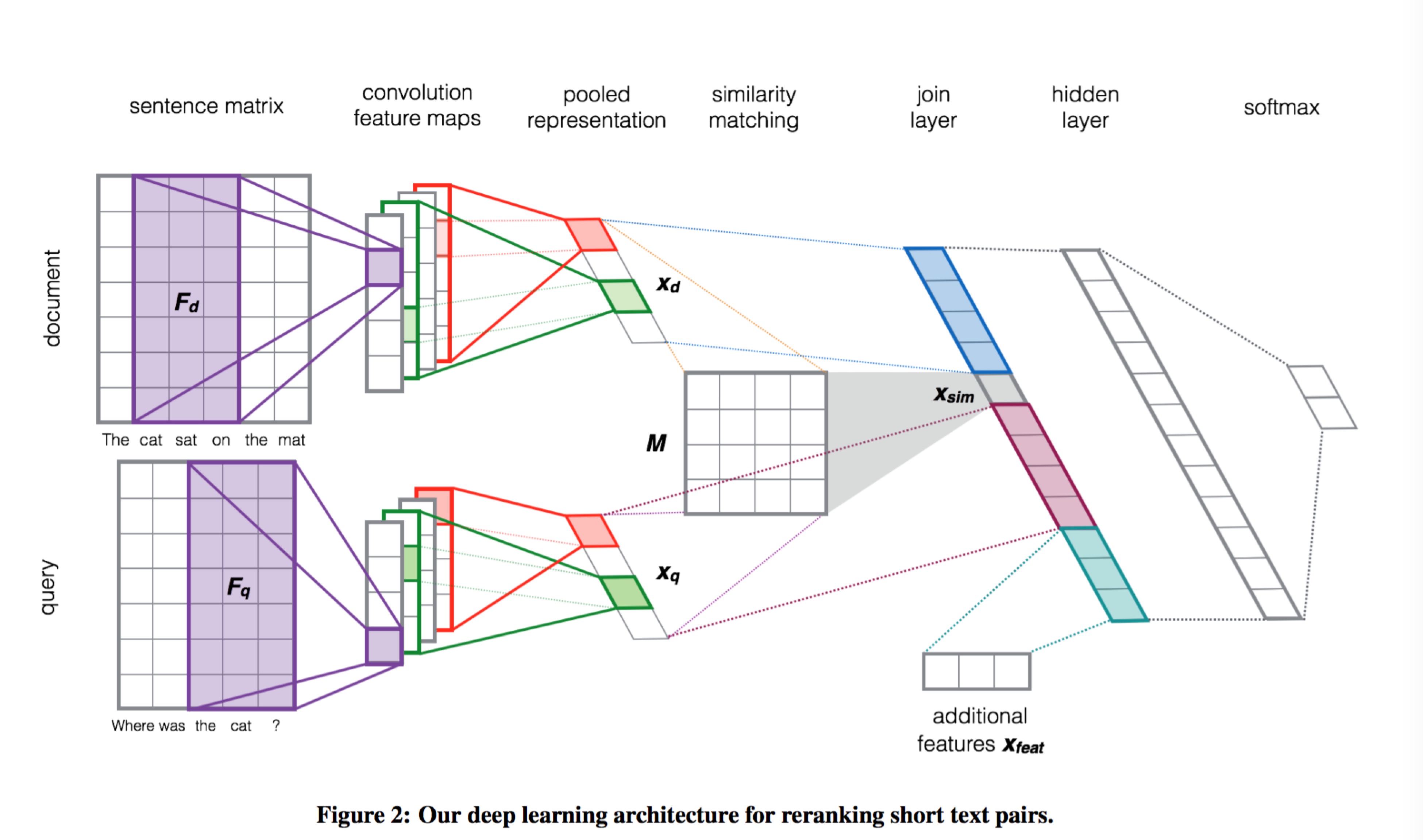
架构? 不能不提到的论文中经典的架构图。
question answer并行处理成词向量
词向量与卷积核做运算得到n个len(q or a)维的向量
对2中得到的向量做Activation和Pooling处理,得到1维数组,大小为n
问题和答案抽出的1维数组分别与相似度矩阵M做乘积预算,得到相似度,即 $A*M*Q=sim$
计算answer和question中的相同部分F,将A,sim,Q,F拼接成新的向量
将5中得到的向量做线性变化,即 $\alpha(W*X+b)$
最后使用Softmax对6中得到的linear之后的向量做分类
使用theano的实现 作者的实现有一些改动,如第5步骤中计算得到的交叉部分F,这部分可以是交叉词的词向量,也可以是交叉词的idf,比重等,显然idf和比重更容易让人信服,不过这个值不好处理,作者并没有用,而是直接使用的交叉词的词向量拼到question和answer的词向量中,即将这部分直接放到开头做了。
数据预处理(embedding) 这部分主要是将question-answer对分词(英文就是空格直接分词), 然后根据word2vec,将问题和答案分解成word2vec的词向量,并收集全集词表,word2vec缺失的词使用默认值填充。难点在于训练集合的选取,这是有监督的学习,对于中文的海量语法来说,需要的训练集合的规模也是非常大的。
Load 主要load的数据有train, dev, test三类,train是训练参数使用,dev是验证参数,test是实测使用,其实dev和test可以归为一类,每类数据分为question, answer, overlap。
词向量转化 LookupTableFast将question, answer, overlap转化为词向量。这里会讲pad部分(即卷积的宽度补上),最后输出的是 [batch_size, 1, 2 * (q_size + q_filter_widths - 1), ndim], ndim是词向量的宽度(word2vec生成的词向量的size),后面ndim的长度会拓展为1
2
# sentence长度 + 交叉长度
ndim = vocab_emb.shape[1] + vocab_emb_overlap.shape[1]
1
2
3
4
5
6
7
8
9
10
11
12
13
14
15
class LookupTableFastStatic(Layer):
def __init__(self, W=None, pad=None):
super(LookupTableFastStatic, self).__init__()
self.pad = pad
self.W = theano.shared(value=W, name='W_emb', borrow=True)
def output_func(self, input):
out = self.W[input.flatten()].reshape((input.shape[0], 1, input.shape[1], self.W.shape[1]))
if self.pad:
pad_matrix = T.zeros((out.shape[0], out.shape[1], self.pad, out.shape[3]))
out = T.concatenate([pad_matrix, out, pad_matrix], axis=2)
return out
def __repr__(self):
return "{}: {}".format(self.__class__.__name__, self.W.shape.eval())
卷积 定义Conv2dLayer来做卷积类使用,卷积的初始化如下1
2
3
4
5
def __init__(self, rng, filter_shape, input_shape=None, W=None):
# @rng: 初始化种子
# @filter_shape: 卷积核的样式,filter_shape = (nkernels, num_input_channels, filter_width, ndim), nkernels = 100, num_input_channels = 1, 可见与question长度无关。
# @input_shape: 同上一层词向量层的输出
# @self.W 也和filter_shape具有相同的shape,随机化一些数字
卷积使用库函数,调用如下1
2
3
4
def output_func(self, input):
return conv.conv2d(input, self.W, border_mode='valid',
filter_shape=self.filter_shape,
image_shape=self.input_shape)
看看conv2d函数的返回, 看到output的是 [batch_size, filter_size, sentence_size, ndim]1
2
3
4
5
6
7
8
9
10
Parameters:
input (dmatrix of dtensor3) – Symbolic variable for images to be filtered.
filters (dmatrix of dtensor3) – Symbolic variable containing filter values.
border_mode ({'valid', 'full'}) – See scipy.signal.convolve2d.
subsample – Factor by which to subsample output.
image_shape (tuple of length 2 or 3) – ([number images,] image height, image width).
filter_shape (tuple of length 2 or 3) – ([number filters,] filter height, filter width).
kwargs – See theano.tensor.nnet.conv.conv2d.
Returns:
Tensor of filtered images, with shape ([number images,] [number filters,] image height, image width)
何为卷积?如何卷积?
cnn的核心在于卷积核,其实关于卷积核还有另一个名字叫做滤波器,从信号处理的角度而言,滤波器是对信号做频率筛选,这里主要是空间-频率的转换,cnn的训练就是找到最好的滤波器使得滤波后的信号更容易分类,还可以从模版匹配的角度看卷积,每个卷积核都可以看成一个特征模版,训练就是为了找到最适合分类的特征模板。
卷积核最后是作为最终的feature,每个卷积核作为一个特征,与question、answer等都无关了,所以卷积核的特征采集是非常重要的。
$$
Activation (tanh) 使用nn_layers.NonLinearityLayer作为主类,初始化以及output函数:1
2
3
4
NonLinearityLayer(b_size=filter_shape[0], activation=activation)
def output_func(self, input):
return self.activation(input + self.b.dimshuffle('x', 0, 'x', 'x'))
dimshuffle是将b拓展到4维,正好与卷积的output匹配相加。这里有一个问题,卷积出的第四维度是ndim,和公式算的$c_i$没有该维度,该维度上直接相加了。
Pooling 1
2
3
# 在第二维度上,即image height,也就是sentence
def max_pooling(input):
return T.max(input, axis=2)
PairwiseNoFeatsLayer 这个是将q和a经过上面一系列的层产生的结果(最后是经过Pooling处理得到的[batch_size, n])做乘积,求q和a的相似性sim,最后将q,a,sim拼接。1
2
3
4
5
6
7
8
# 注意这里的参数W矩阵是(n * n)的
def output_func(self, input):
# P(Y|X) = softmax(W.X + b)
q, a = input[0], input[1]
# dot = T.batched_dot(q, T.batched_dot(a, self.W))
dot = T.batched_dot(q, T.dot(a, self.W.T))
out = T.concatenate([dot.dimshuffle(0, 'x'), q, a], axis=1)
return out
out的长度为q_logistic_n_in + a_logistic_n_in + 1
LinearLayer 线性变换,这里的输入是长度为q_logistic_n_in + a_logistic_n_in + 1的特征数组,需要经过线性变化,LinearLayer1
2
3
# W是(q_logistic_n_in + a_logistic_n_in + 1) * (q_logistic_n_in + a_logistic_n_in + 1)
def output_func(self, input):
return self.activation(T.dot(input, self.W) + self.b)
LogisticRegression 最后一步,上面的输入仍然是q_logistic_n_in + a_logistic_n_in + 1, 使用softmax输出求解,1
2
3
4
5
def output_func(self, input):
# P(Y|X) = softmax(W.X + b)
self.p_y_given_x = T.nnet.softmax(self._dot(input, self.W) + self.b)
self.y_pred = T.argmax(self.p_y_given_x, axis=1)
return self.y_pred
注意T.argmax是获取下标,所以这里的输出是直接分类(本问题中是0,1), p_y_given_x是给的具体的概率值。
训练网络 前面的整个网络已经布局完毕,是计算loss的时候了,cost=negative_log_likelihood(y)=-T.mean(T.log(self.p_y_given_x)[T.arange(y.shape[0]), y]), 使用adadelta训练参数,这个cost如何理解呢?找到了解释,我自己是没有跑通,囧。1
2
3
4
5
6
7
8
9
10
11
# y.shape[0] is (symbolically) the number of rows in y, i.e.,
# number of examples (call it n) in the minibatch
# T.arange(y.shape[0]) is a symbolic vector which will contain
# [0,1,2,... n-1] T.log(self.p_y_given_x) is a matrix of
# Log-Probabilities (call it LP) with one row per example and
# one column per class LP[T.arange(y.shape[0]),y] is a vector
# v containing [LP[0,y[0]], LP[1,y[1]], LP[2,y[2]], ...,
# LP[n-1,y[n-1]]] and T.mean(LP[T.arange(y.shape[0]),y]) is
# the mean (across minibatch examples) of the elements in v,
# i.e., the mean log-likelihood across the minibatch.
return -T.mean(T.log(self.p_y_given_x)[T.arange(y.shape[0]), y])
如何更新参数呢?1
updates = sgd_trainer.get_adadelta_updates(cost, params, rho=0.95, eps=1e-6, max_norm=max_norm, word_vec_name='W_emb')
作者实现的adadelta算法如下所示, 加上了我自己的理解和注释,我感觉这块的实现有些问题,因为adadelta是前t次的迭代,而这里的和显然是从开始到结束,有点像adagrad。后面贴的链接是几种求参迭代的方法。1
2
3
4
5
6
7
8
9
10
11
12
13
14
15
16
17
18
19
20
21
22
23
24
25
26
27
28
29
30
31
32
33
34
35
36
37
38
39
40
41
42
43
44
45
46
def get_adadelta_updates(cost, params, rho=0.95, eps=1e-6, max_norm=9, word_vec_name='W_emb'):
print "Generating adadelta updates"
updates = OrderedDict({})
exp_sqr_grads = OrderedDict({})
exp_sqr_ups = OrderedDict({})
gparams = []
# 这里设置了三个变量, for every param:
# exp_sqr_grads init zeros
# exp_sqr_ups zeros
# gparams [] list append gp(grad)
for param in params:
exp_sqr_grads[param] = build_shared_zeros(param.shape.eval(), name="exp_grad_%s" % param.name)
print 'cost ', cost
print 'param.shape.eval', param.shape.eval()
gp = T.grad(cost, param)
print 'gp', gp
exp_sqr_ups[param] = build_shared_zeros(param.shape.eval(), name="exp_grad_%s" % param.name)
print 'exp_sqr_ups', exp_sqr_ups[param].shape
gparams.append(gp)
print param, gp
#真正的计算, for every param
# exp_sg 之前的 sum(sqr(gp) 1...t-1) for now param
# exp_su 之前的 sum(step 1...t-1) for now param
# up_exp_sg = rho * exp_sg + (1 - rho) * T.sqr(gp); 加上现在的gp平方
# updates[exp_sg] = up_exp_sg 换上
# step = -(T.sqrt(exp_su + eps) / T.sqrt(up_exp_sg + eps)) * gp,该次更新的param step,
注意这里分母的gp是1..t,而分子的sum(step)是 1...t-1
#updates[exp_su] = rho * exp_su + (1 - rho) * T.sqr(step); 更新本次
#stepped_param = param + step;最后目标
for param, gp in zip(params, gparams):
exp_sg = exp_sqr_grads[param]
exp_su = exp_sqr_ups[param]
up_exp_sg = rho * exp_sg + (1 - rho) * T.sqr(gp)
updates[exp_sg] = up_exp_sg
step = -(T.sqrt(exp_su + eps) / T.sqrt(up_exp_sg + eps)) * gp
updates[exp_su] = rho * exp_su + (1 - rho) * T.sqr(step)
stepped_param = param + step
# if (param.get_value(borrow=True).ndim == 2) and (param.name != word_vec_name):
if max_norm and param.name != word_vec_name:
col_norms = T.sqrt(T.sum(T.sqr(stepped_param), axis=0))
desired_norms = T.clip(col_norms, 0, T.sqrt(max_norm))
scale = desired_norms / (1e-7 + col_norms)
updates[param] = stepped_param * scale
else:
updates[param] = stepped_param
return updates
参考资料:http://blog.csdn.net/luo123n/article/details/48239963 http://sebastianruder.com/optimizing-gradient-descent/index.html#gradientdescentvariants http://www.cnblogs.com/neopenx/p/4768388.html http://deeplearning.net/tutorial/code/lstm.py